
5 Recruits
The four Cardinal Virtues for working through a data science problem are Wisdom, Justice, Courage, and Temperance. This chapter — the first example chapter in the Primer — works through the simplest possible problem the four virtues have to handle: a predictive linear regression with one binary covariate. The matching tutorial is 06-recruits in the primer.tutorials package; almost every line of code in that tutorial appears here, surrounded by more prose, more exploration, and a paired causal version of the same question.
Imagine that you are a logistics analyst at U.S. Marine Corps Supply, planning next year’s bootcamp uniform order. The Quartermaster General has a big-picture goal — every recruit kitted out at the right size on day one, within a fixed procurement budget — and many decisions to make in service of it: how many uniforms to purchase, from which vendors, in which fabrics, in which sizes, and how many of each size to hold in inventory against the unexpected. The Quartermaster has not asked you for a “causal estimate” or a “predictive model”; those words don’t appear in the procurement plan. What the Quartermaster asks for is evidence that helps with the decisions. This chapter focuses on one such piece of evidence: an estimate of the average height of male and female recruits expected to enlist next year, with its associated uncertainty. The estimate alone won’t determine the order, but it is one good input. There are many decisions to make.
The data we will work from is recruits, a 50-row teaching cut of NHANES (the National Health and Nutrition Examination Survey, conducted by the U.S. Centers for Disease Control and Prevention). It has three columns: height (centimeters), sex (Female / Male), and age (integer years, restricted to 18–27). The 40 male and 10 female rows are deliberately unbalanced — a feature we will return to when we look at the model’s standard errors.
5.1 Wisdom
Wisdom begins with a question and then moves on to the creation of a Preceptor Table and an examination of our data.
Wisdom commits us to a question that is precise enough to be answered. The Preceptor Table makes the commitment concrete: it is the smallest table that, if every cell were filled in with the truth, would make the question’s answer easy to read off.
The combination of some data and an aching desire for an answer does not ensure that a reasonable answer can be extracted from a given body of data. — John W. Tukey
5.1.1 The Marine Corps and the supply problem
The U.S. Marine Corps takes in roughly 25,000 to 30,000 enlisted recruits each year, training them at one of two depots: Marine Corps Recruit Depot Parris Island in South Carolina (recruits from east of the Mississippi, plus all female recruits since 2019) and MCRD San Diego in California (men from west of the Mississippi). Recruits arrive for a 13-week training program. On day one, each new recruit is issued a “sea bag” — a duffel of basic clothing and equipment including dress uniforms, utility uniforms (cammies), physical training gear, footwear, and headgear, all in sizes determined before the recruit walked through the door.
The supply chain has to forecast the size mix in advance. The forecast can go wrong in either direction: too many extra-large jackets and the surplus sits in inventory; too few and recruits wait, schedules slip, and money is wasted on rush orders. The cost of a bad forecast is not negligible — the Marine Corps spends a few hundred dollars per recruit on basic-issue gear, multiplied across tens of thousands of recruits a year. The Quartermaster’s question is therefore concrete: how many of each size? Among the inputs to that forecast is the height distribution of incoming recruits, broken out by sex — which is what this chapter estimates.
A few features of the recruit population matter for what comes later. Recruits must clear a fitness screen and meet height/weight standards before enlistment, so the recruit population is not a random sample of U.S. young adults. The male-female ratio in the Marine Corps is heavily skewed (active-duty enlisted is about 91% male, 9% female), and the geographic origin of recruits varies (more than half come from the southern United States). All of these facts will come back when we discuss representativeness in Justice.
5.1.2 NHANES, the data source
The data we use comes from the National Health and Nutrition Examination Survey (NHANES), the continuous version of an examination survey the National Center for Health Statistics has run since the early 1960s. NHANES draws a stratified, multistage probability sample from the U.S. civilian noninstitutionalized population, oversampling specific demographic groups — older adults, racial and ethnic minorities, lower-income households — so that subgroup estimates have adequate precision. Selected participants are interviewed at home and then visited at a Mobile Examination Center, a fleet of medical-grade trailers that travels around the country. Examiners measure height, weight, blood pressure, and a battery of other physical measurements; trained phlebotomists draw blood. Since 1999, NHANES has examined roughly 5,000 individuals per year and reports results in two-year cycles.
The recruits tibble used in this chapter is a 50-row teaching cut drawn from the much larger NHANES file, restricted to ages 18–27 with non-missing height and sex, with the male-female split deliberately set to 40/10 to make the standard-error contrast visible later. The 40/10 split is not representative of the actual demographic mix of NHANES participants in this age range, and the educational version of NHANES that the cut is drawn from drops the survey weights that would let us reweight back to a representative sample.
Two features of how NHANES measures height matter. First, height is recorded by a trained examiner using a fixed stadiometer, with the participant standing barefoot, heels together, head positioned to a standard plane. Second, the examination happens in a controlled clinical setting — the same procedure for every participant, repeatable across years. Both features will return in the validity discussion in Justice, where we ask whether NHANES heights and USMC enlistment heights measure the same construct.
5.1.3 The primary question
The primary question for this chapter is predictive:
What will be the average height of male and female USMC recruits next year?
This is a predictive question — the kind of question that calls for a predictive model. We want two specific numbers: an estimate of the average height of male recruits next year, and an estimate of the average height of female recruits next year, each with its uncertainty. The Preceptor Table that would let us answer it directly has three columns — one identifying each recruit, one for height, and one for sex — and one row per USMC recruit expected to enlist next year (the 25,000-to-30,000 figure cited above).
A note on language. Average height and expected height are not the same thing. The average height of next year’s recruits is a real physical fact: line up everyone who shows up, measure each one, divide by the count, and you have a number. We will not have those measurements (those recruits have not shown up yet), so we cannot compute the average directly. What our model will produce is an expected height — the model’s best guess of what the average should be, given our data and our assumptions. Expected and average are not the same; we will return to that distinction in later chapters. For now, the Preceptor Table is about averages we cannot directly observe; the model is about expected values that approximate them.
| Preceptor Table --- Primary (predictive) question1 | ||
| Recruit | Height (cm) | Sex |
|---|---|---|
| 1 If all the information in this table were available, we could answer the question: What will be the average height of male and female USMC recruits next year? | ||
| 2 Each row is one USMC recruit expected to enlist during the coming year, about 25,000 to 30,000 recruits in total. | ||
| 3 Height in centimeters, measured at enlistment. | ||
| 4 Sex, taking values 'Male' or 'Female', as recorded at enlistment. | ||
The Preceptor Table is imaginary in the sense that we will never have its full content; even our 50-row sample will only let us guess at the missing cells. But the act of writing it down is what forces the question to be precise. The smallest table that would answer the question is exactly three columns wide and 25,000-to-30,000 rows tall. Anything more is irrelevant; anything less and the question is unanswerable.
5.1.4 Exploring the data
Before fitting a model, look at the data. You can never look too closely at your data — the hour spent on a careful EDA almost always saves a day downstream.
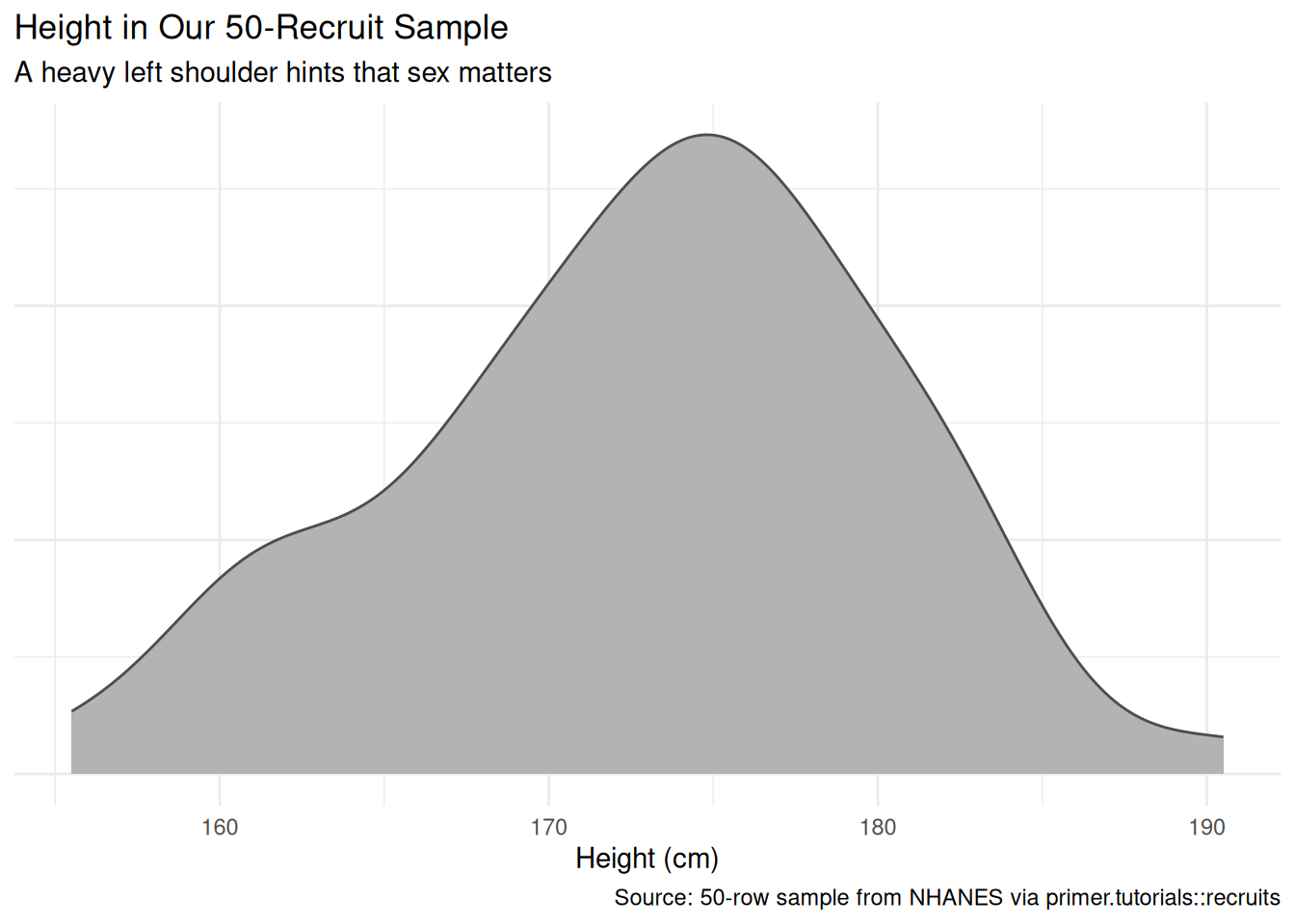
The marginal distribution of height has a left shoulder near 162 cm and a main mass near 175 cm. The shoulder is hinting that the sample is not unimodal; splitting by sex confirms it.
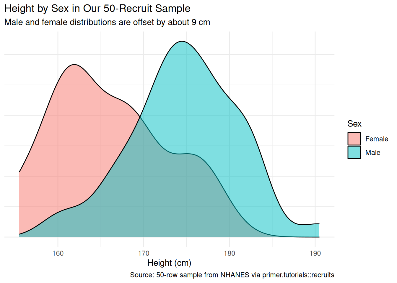
The female distribution sits visibly to the left of the male distribution, with the female mode near 162 cm and the male mode near 175 cm — about a 13 cm offset at the modes, with substantial overlap in the tails. The female density also looks rougher because we have only 10 female rows; a density estimator with 10 observations is wobbly.
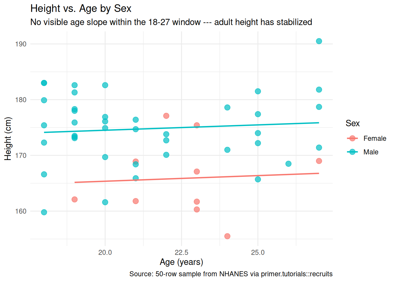
Plotting height against age, separately for male and female, shows essentially no slope on age within the 18–27 window. This makes biological sense: human height stops growing in the late teens. We will keep age in mind as a candidate covariate during Courage but should not be surprised when it adds nothing to the model.
A few specifics worth flagging from the EDA:
- The 40/10 male/female split is not nationally representative. Real USMC recruits are roughly 90% male and 10% female; our 80/20 sample is somewhere between that recruit reality and an even split. The unbalanced sample means the male group’s mean estimate will be much more precise than the female group’s — a feature we will see surfaced in the standard errors.
-
No missing values. The packaged
recruitstibble has been cleaned; there is no NA-handling work to do. - The age range is narrow (18–27), so the height distribution can be treated as the adult-height distribution for this exercise.
5.1.5 The paired question
The difference between predictive models and causal models is that the former have one column for the outcome variable and the latter have more than one column.
Every chapter pairs its primary question with one in the opposite framing. Since our primary question is predictive, the paired question is causal:
What is the causal effect of sex on a recruit’s height?
This is a deliberately absurd question. Sex is not a manipulable variable: you cannot toggle a recruit’s sex and watch their height change. A genuine causal interpretation would require us to compare a single recruit’s height under two counterfactual histories — one where they were assigned female, one where they were assigned male — which has no operational meaning.
The reason we ask the absurd question anyway is to make a point. The same fitted model serves both framings. The same number (\(\beta_1 \approx 9\) cm) is the answer to both. What differs is the analyst’s commitment:
- The predictive reading describes a comparison between two groups: when we compare two recruits differing only in sex, the male recruit has an expected height about 9 cm taller than the female recruit. This is a statement about averages, not about any individual.
- The causal reading would describe an effect: changing a recruit’s sex from female to male would increase their expected height by about 9 cm. This requires a counterfactual we cannot construct.
The predictive reading is honest. The causal reading is mostly pedagogical: it shows that the predictive/causal distinction is something the analyst commits to, not something the data forces. With sex and height, the causal reading is absurd; with the exact same fit, a different problem might support a defensible causal reading. The point of writing both Preceptor Tables for this chapter is to make that visible.
| Preceptor Table --- Paired (causal) question1 | |||
| Recruit | Height if Female | Height if Male | Sex |
|---|---|---|---|
| 1 If all the information in this table were available, we could answer the question: What is the causal effect of sex on a recruit's height? The implied manipulation (toggling a recruit's sex) is not realizable; the table is a pedagogical device, not a defensible causal claim. | |||
| 2 Each row is one USMC recruit. Same units as the primary Preceptor Table. | |||
| 3 Each row's cross-hatched cell marks the unobservable counterfactual --- the height the recruit would have had under the sex they were not assigned. The truth would exist if the counterfactual existed; nothing in reality could ever reveal it. | |||
| 4 The treatment is the recruit's actual sex. Putting it under a Treatment spanner is what marks this table as causal; in the primary Preceptor Table the same column sat under a Covariate spanner. | |||
Compare the two Preceptor Tables side by side. Almost everything is the same: same units, same row count, same role of Recruit as the unit identifier. The two structural differences are exactly the bookkeeping of the predictive/causal split:
- The primary table has one outcome column (
Height (cm)); the paired table has two potential-outcome columns (Height if Female,Height if Male), one per value of the treatment, with the unobservable counterfactual hatched. - The primary table has the
Sexcolumn under a Covariate spanner; the paired table has the same column under a Treatment spanner. The column itself is identical. Only the spanner — the analyst’s commitment — changed.
The same fitted model serves both questions. The chapter’s two Temperance answers will read the same number through the two framings.
5.2 Justice

Justice concerns the Population Table, the four key assumptions which underlie it (validity, stability, representativeness, and unconfoundedness), and the choice of probability family and link function for the data generating mechanism.
Justice is the section of the analysis where you (or your critics) raise concerns about whether the model will do what you want it to do — and where you commit to defending it. The four assumptions are the named families of concerns. They are not testable from the data alone; they are choices the analyst makes and defends.
The bridge runs in one direction: data → population → Preceptor Table. The data tells us about the population from which both the data and the Preceptor Table are drawn; the population tells us about the Preceptor Table’s units. Justice’s job is to make sure both arrows are defensible.
There are known knowns. There are things we know we know. We also know there are known unknowns. That is to say, we know there are some things we do not know. But there are also unknown unknowns, the ones we do not know we do not know. — Donald Rumsfeld
5.2.1 The Population Table for the primary question
| Population Table --- Primary question1 | ||||
| Young Adult | Year | Height (cm) | Sex | |
|---|---|---|---|---|
| 1 Data rows are 50 NHANES respondents aged 18-27, examined between 1999 and the most recent release. Preceptor rows are the 25,000-to-30,000 USMC recruits expected to enlist in 2026. The two blocks share the broader population of US young adults aged 18-27 but differ in era, in self-selection, and in measurement procedure. | ||||
5.2.2 Validity
Validity is the consistency, or lack thereof, in the columns of the data set and the corresponding columns in the Preceptor Table.
Validity is about columns. Two columns can have the same name and still measure different things; two columns can have different names and still measure the same thing.
For our problem, both height columns are labeled “Height (cm)” but the measurement procedures differ. NHANES heights are measured in the Mobile Examination Center by trained examiners using a fixed stadiometer, with shoes removed, instructions standardized across all participants. USMC heights are recorded at the recruiting office or at bootcamp intake, with whatever stadiometer is available, possibly with shoes on, possibly with whatever instructional drift has accumulated since the last standardization. A systematic offset of a centimeter or two between the two procedures would not be surprising.
That difference in measurement procedure means our height column in the data may not be exactly the same construct as our height column in the Preceptor Table. We commit to the assumption that the two are close enough — that the Preceptor Table’s hypothetical “true” recruit heights are well-approximated by NHANES adult heights for the same demographic group — but a critic could push back here, and the model’s standard errors do not capture that critic’s worry.
5.2.3 Stability
Stability means that the relationship between the columns in the Population Table is the same for three categories of rows: the data, the Preceptor Table, and the larger population from which both are drawn.
Stability is a statement about parameters, not distributions. A change in the marginal distribution of height between 2002 and 2026 does not, by itself, violate stability. What violates stability is a change in the parameters governing the relationship: the intercept, the slope on sexMale, the residual variance.
For Recruits, the relevant stability worry is small. Adult human height has been stable for the broad U.S. young-adult population for several decades — the intercept may have drifted upward by a centimeter or two as nutrition has improved, but the male-female height gap (the parameter we care about most) has barely moved. We commit to stability and move on.
A common confusion is to point at any change between two eras and call it a stability violation. It isn’t. The mean of height in the population may have shifted upward; the spread of heights may have narrowed; the mix of ethnicities in the recruiting pool may differ from NHANES participants. None of those, on their own, is a stability violation. Stability requires that \(\beta_0\) and \(\beta_1\) stay put. Distribution shifts are everywhere; parameter shifts are what hurt us.
5.2.4 Representativeness
Representativeness, or the lack thereof, concerns two relationships among the rows in the Population Table. The first is between the data and the other rows. The second is between the other rows and the Preceptor Table.
Two links to defend.
Data → population. NHANES is closer to a probability sample than most U.S. health surveys — it is a stratified, multistage probability sample drawn from the U.S. civilian non-institutionalized population. But the educational version of NHANES that we draw recruits from drops the survey weights, and our 50-row sample further skews the male-female split to 40/10 (deliberately, to make the standard-error contrast visible later). So our data block is not a random sample of U.S. young adults; it is closer to “U.S. young adults in the educational NHANES file, with female respondents under-represented relative to male.” A non-representative sample doesn’t guarantee a biased estimate — the bias might wash out by chance — but chance is the only mechanism left to defend us, and we have no principled reason to expect it to work in our favor.
Population → Preceptor Table. USMC recruits are not a random sample of U.S. young adults. They are self-selected (volunteers), screened for fitness (filtering out ineligible applicants), and skewed toward demographics historically over-represented in the military. The recruits we will be ordering uniforms for are very likely taller on average than NHANES participants of the same age range, both because the fitness screen filters out shorter applicants at the bottom of the pool and because the recruit population’s demographic mix differs from the U.S. average. The model’s intercept and slope, fit to NHANES, will probably understate recruit height by a centimeter or two.
5.2.5 Unconfoundedness (paired causal question only)
Unconfoundedness means that the treatment assignment is independent of the potential outcomes, when we condition on pre-treatment covariates.
Unconfoundedness applies only to the paired causal question. For the primary predictive question we don’t even ask — predictive models have no treatment, so the assumption is not relevant.
For the paired causal question, unconfoundedness is not defensible. Sex assignment is not a manipulable treatment; there is no randomization mechanism, no plausible defense of “treatment assignment independent of potential outcomes.” If we wrote down the treatment assignment mechanism, we would have to write something biological, deterministic, and confounded with thousands of unobserved variables (genetics, hormonal exposure in utero, and so on, all of which also affect adult height through pathways that have nothing to do with the proximate “treatment”). The unconfoundedness assumption fails.
This is the substantive reason the paired causal question is absurd, not just rhetorical. We carry the paired Preceptor Table through the chapter to show what the bookkeeping would look like if we made the causal commitment, but Temperance’s causal reading will not be defensible as a causal claim about the world. It is defensible only as a translation exercise — “if we made these assumptions, here is what the model would say” — which is a useful pedagogical move but not a useful policy claim.
5.2.6 The Population Table for the paired question
The paired Population Table has the same row structure as the primary — 50 NHANES Data rows and 25,000-to-30,000 Preceptor rows — but two outcome columns instead of one (Height if Female, Height if Male). In Data rows, the unobserved counterfactual is .... In Preceptor rows, both potential outcomes are filled in, with the unobservable one hatched.
| Population Table --- Paired (causal) question1 | |||||
| Young Adult | Year | Height if Female | Height if Male | Sex | |
|---|---|---|---|---|---|
| 1 Same row structure as the primary Population Table, with two outcome columns instead of one. In Data rows, only one potential outcome is observed --- the one matching the recruit's actual sex; the counterfactual is '...' because no empirical process recorded it. In Preceptor rows, both potential outcomes are filled in; the unobservable counterfactual is hatched. | |||||
The two Population Tables differ in exactly the same way the two Preceptor Tables did: one outcome column versus two, with hatching and ... notation in the causal version to handle the unobservable counterfactual.
5.2.7 Probability family and link function
The probability family is determined by the outcome’s distribution. height is continuous, so the family is Normal:
\[Y \sim \mathcal{N}(\mu, \sigma^2)\]
The link function for a continuous outcome is the identity, so:
\[\mu = \beta_0 + \beta_1 X_1 + \cdots + \beta_n X_n\]
Our model will be a linear regression. The covariates we will use are determined in Courage.
5.3 Courage

Courage creates the data generating mechanism.
The three languages of data science are words, math, and code, and the most important of these is code. Justice settled the structural choices — continuous outcome, Normal family, identity link. Courage now picks specific covariates, writes the model formula in code, and uses R to estimate the unknown parameters.
The abstract DGM coming out of Justice is:
\[Y = \beta_0 + \beta_1 X_1 + \beta_2 X_2 + \cdots + \beta_n X_n + \epsilon\]
with \(\epsilon \sim \mathcal{N}(0, \sigma^2)\).
5.3.1 Candidate models
Courage almost never settles on its first guess. We try a handful of plausible specifications, look at what each says, and commit to the one that matches the question.
5.3.1.1 Candidate 1: height ~ sex
| term | estimate | conf.low | conf.high |
|---|---|---|---|
| (Intercept) | 165.9 | 161.8 | 170.0 |
| sexMale | 8.9 | 4.3 | 13.4 |
The intercept is the expected height of a female recruit (the reference level): about 165.9 cm. The slope on sexMale is about 8.9 cm: when we compare two recruits differing only in sex, the male recruit is expected to be 8.9 cm taller. The 95% confidence interval for sexMale is roughly [4.3, 13.4]; zero is well outside that interval, so the model says the expected height of male recruits is taller than the expected height of female recruits. That does not mean every male is taller than every female — the two distributions overlap, and there are plenty of female recruits taller than some male recruits.
Notice the language: “when we compare two recruits differing only in sex”. For a binary covariate the comparison framing is the only honest reading of a predictive model. We do not say “raising sex by one unit increases height by 8.9 cm” because raising sex is not a thing.
5.3.1.2 Candidate 2: height ~ age
| term | estimate | conf.low | conf.high |
|---|---|---|---|
| (Intercept) | 173.5 | 157.7 | 189.2 |
| age | 0.0 | -0.7 | 0.7 |
The slope on age is essentially zero, with a 95% confidence interval that crosses zero in both directions. Comparing two recruits differing by one year of age (within our 18–27 window), their expected heights are indistinguishable. Adult height has stopped changing by the late teens; this fit confirms it. We had already anticipated this from the EDA.
5.3.1.3 Candidate 3: height ~ sex + age
| term | estimate | conf.low | conf.high |
|---|---|---|---|
| (Intercept) | 161.5 | 146.4 | 176.6 |
| sexMale | 9.1 | 4.5 | 13.8 |
| age | 0.2 | -0.5 | 0.8 |
Adding age to the sex-only model leaves the sexMale coefficient essentially unchanged (still about 8.9 cm) and confirms that age adds no signal — its coefficient is again indistinguishable from zero. This is exactly what we would expect if age and sex are roughly uncorrelated in our sample (which they are) and if age has no real effect on height in the 18–27 window (which it doesn’t).
5.3.2 The chosen DGM
Adding age does not change the answer to the question we asked. The simpler model is therefore preferable:
With the parameters estimated, we can write the fitted DGM as a concrete formula:
\[\widehat{\text{Height}} = 165.9 + 8.9 \cdot \text{sexMale}\]
Three differences from the abstract form. First, the parameters \(\beta_0\) and \(\beta_1\) are replaced by their best estimates (rounded to one decimal place). Second, the error term is gone because this formula generates our estimated outcome, not a description of its randomness. Third, the left-hand side has a hat (\(\widehat{\text{Height}}\)) because hats indicate estimated values.
sexMale is a 0/1 dummy: 1 for male recruits, 0 for female. Math doesn’t speak text; dummies do the translation. The intercept (165.9) is the expected height of a female recruit; adding the slope (8.9) gives the expected male recruit height of 174.8 cm.
This is our data generating mechanism. We will use it for both the primary and the paired questions in Temperance. The fit object is the same; what differs is how we read it.
5.3.3 Model checking
A simple sanity check: the distribution of the fitted values should look like the distribution of the actual height. They will not match exactly — the model has only two predicted values (one for female, one for male) while the actual data has continuous variation — but the gross shape and central tendency should be close.
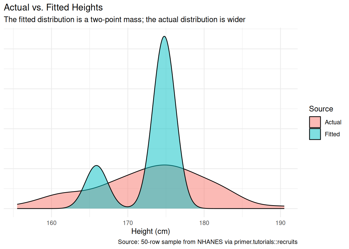
The fitted distribution has two narrow spikes (one near 165.9 cm, one near 174.8 cm) corresponding to the two predicted values. The actual distribution has continuous spread within and between the two groups. The two distributions agree on central tendency and rough shape but differ on spread — which is what we expect from a model that uses only one binary covariate. Adding more covariates (or using a richer functional form) would let the model recover more of the actual spread; for our question, two predicted values is all we need.
5.4 Temperance

Temperance interprets the data generating mechanism and then uses it to answer, with the help of graphics, the question(s) with which we began. Humility reminds us that this answer is always false.
In the modern world, all parameters are nuisance parameters. What we care about is what the model says on the outcome scale: predicted heights, predicted differences. The tool for translating parameters into outcome-scale answers is the marginaleffects package, with companion book Model to Meaning by Vincent Arel-Bundock.
5.4.1 The primary (predictive) reading

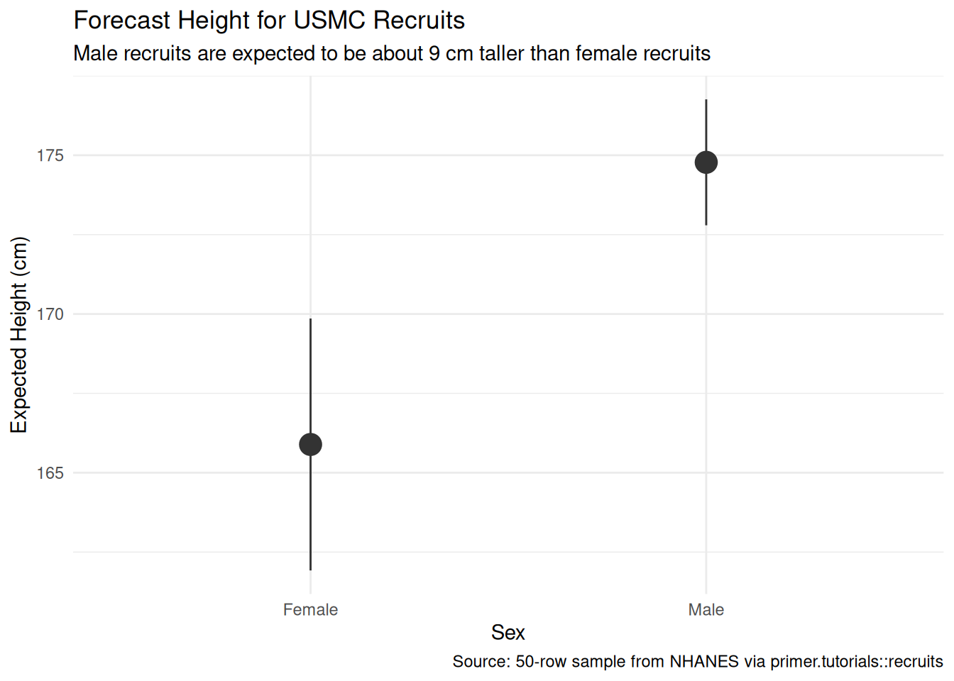
The primary question was “What will be the average height of male and female USMC recruits next year?” The model’s answer:
- The expected height of a male recruit is about 174.8 cm, with a 95% confidence interval of roughly [172.5, 177.0].
- The expected height of a female recruit is about 165.9 cm, with a 95% confidence interval of roughly [161.8, 170.0].
Note that the female interval is visibly wider than the male interval. The standard error of a group mean shrinks roughly with the square root of the group’s sample size, so quadrupling the sample (from 10 female rows to 40 male rows) halves the standard error. The female interval ends up about twice as wide as the male interval — the deliberate 40/10 split in the recruits tibble was designed to make this contrast visible.
The language is comparison language throughout. Comparing two groups of recruits, the male group has expected height 9 cm taller than the female group. No words like cause, raise, change. The model is predictive; the language tracks the framing.
5.4.2 The paired (causal) reading
The paired question was “What is the causal effect of sex on a recruit’s height?” The same fitted model gives the same number: a coefficient of 8.9 cm on sexMale.
The causal reading would say: changing a recruit’s sex from female to male would raise their expected height by about 9 cm. That is what the paired Preceptor Table commits us to. The bookkeeping is fine, the arithmetic is fine, the number is fine. The reading itself is absurd: there is no manipulation that changes a recruit’s sex while leaving the rest of the recruit identical, because so much of the rest of the recruit is downstream of sex (genetics, hormonal exposure, body composition). Unconfoundedness fails by construction.
The pedagogical point is not that the causal reading is true — it isn’t — but that the causal reading is available, in the sense that the same fit and the same number can be read either way. The thing that makes a model causal or predictive is the analyst’s commitment about what the covariates are. The data does not change. The fit does not change. The number does not change. What changes is what the analyst is willing to claim. With sex and height, the predictive claim is honest and the causal claim is not. With other problems — a randomized experiment, for example — the same arithmetic supports both readings, and the causal one becomes the more valuable.
5.4.3 QoI variety
The chapter has answered the specific question we asked: the average height of male and female USMC recruits. That is one question in a family. A campaign-quality answer for the Quartermaster would also want, at minimum:
- The maximum. The Quartermaster doesn’t really care about the average recruit’s height; they care about the tallest recruit, because every recruit needs a uniform that fits. The maximum of 27,000 draws from a Normal distribution with \(\mu \approx 175\) and \(\sigma \approx 6.4\) is about 199 cm — substantially taller than the average. The fitted DGM contains this answer; we just have to ask it.
- The 10th and 90th percentiles. How many extra-small uniforms to keep in inventory, and how many extra-large? The 10th and 90th percentiles of the male and female height distributions tell us where the small and large tails sit. The fitted DGM contains these too.
- Distributions over sample statistics. How tall will the tallest recruit out of a specific batch of three be? This is a question about the maximum of a sample of three draws, which is not a single parameter — it is a distribution. To get the answer we simulate from the DGM: draw three synthetic recruits, record the maximum, repeat ten thousand times, build a histogram. The DGM is a generator; once we have it, any question we can phrase as “draw n units, compute statistic, repeat” has an answer.
The point is that “average” is one question in a family, and the DGM answers the whole family once you know how to ask. The chapter does not work through the simulation step in detail — that is for later chapters — but the pattern (draw from the DGM, summarize, repeat) is the general mechanism by which the Rubin framework answers any quantity of interest.
5.4.4 Why the answer is wrong
We can never know the truth.
Three things are likely wrong with our answer.
First, USMC recruits are taller than the general young-adult population NHANES samples from. The fitness screen filters out applicants at the bottom of the height distribution, and the recruit demographics differ from NHANES demographics. Both pull the true recruit-height distribution to the right of what NHANES sees. A defensible point estimate would nudge male recruit heights upward by a centimeter or two and female recruit heights similarly; a defensible confidence interval would be wider than what the model reports.
Second, our 50-row sample is small (only 10 female rows). The female interval reported by the model is correct under the model’s assumptions, but the model’s assumptions don’t capture the validity gap (different measurement procedure) or the representativeness gap (NHANES self-selection plus our sample’s non-random subsample). A real-world consumer of this estimate should widen the female interval by at least 50%.
Third, the world is always more uncertain than our models would have us believe. Even if every assumption we made about validity, stability, and representativeness were exactly right — which they aren’t — the reported posterior would only be the Preceptor’s Posterior, the best posterior achievable under our assumptions, and that is not the truth. The reported confidence intervals capture only sampling uncertainty under the model; they do not capture uncertainty about whether the model itself is correct. The map is not the territory. A clean graphic tells a story, but the story always rests on assumptions that are at best approximately true.
5.5 Summary
People vary in height, and that variation is strongly patterned by sex. Using a 50-row teaching sample drawn from the National Health and Nutrition Examination Survey (NHANES, conducted by the U.S. Centers for Disease Control and Prevention), we estimated the average height of male and female USMC recruits expected to enlist next year. We modeled height as a normally distributed variable which is a linear function of sex, and read the fit two ways: a predictive comparison between male and female recruits, and an absurd-but-pedagogically-useful causal counterfactual that asked what would happen to a recruit’s height under the opposite sex. Both readings used the same fit and the same number; what differed was the analyst’s commitment. The estimate: male recruits about 174.8 cm on average, female recruits about 165.9 cm, with the female confidence interval visibly wider because there are only ten female rows in the sample. Validity, stability, and representativeness all have soft tells against us — the NHANES measurement procedure differs from the USMC procedure, the time gap between data and recruits is wide, and recruits are non-randomly drawn from the broader young-adult population — so the reported estimates probably understate male and female recruit heights by a centimeter or two and the confidence intervals are too narrow.
The number alone won’t determine the Quartermaster’s order. The maximum, the percentiles, and the distribution of sample-level statistics — all available from the same DGM, by simulation if not by direct closed-form — would round out a campaign-quality answer.
The world is always more uncertain than our models would have us believe.